Step 3 — Defining your observing strategy —
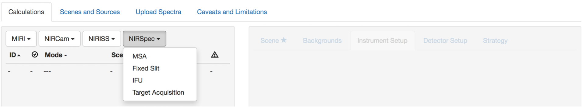
We now explore the options offered by the Calculations thumbnail. At this point, note that you should also consider some trial and error tests in the APT alongside your working with the ETC, so to get an idea of the overheads related to your observations, and adjust the overall execution time to the most efficient strategy. We are going to discuss NIRSpec configurations only: Target Acquisition, IFU and Fixed Slit.
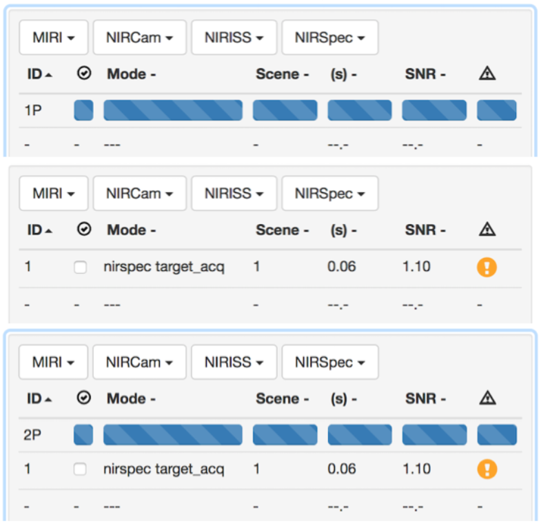
- Select one: ETC may take some time to think.
- It gets an ID, and generic characteristics like duration and SNR which change as you refine the strategy.
- You can add as many configurations as required, including configurations from different instruments.
We start with an IFU configuration (here ID 2), so to explore all the parameters involved in the calculation.
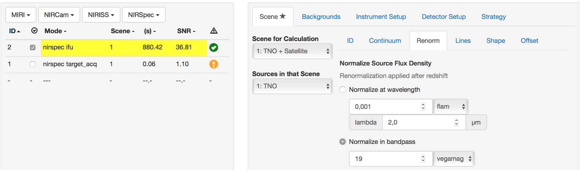
Scene
Select the calculation that you want to modify. Under Scene on the right-hand side of the screen, you can find all the information that were mentioned in the Step 2 – Defining your targets. You can thus modify the target information through this thumbnail too.
If you have defined several scenes in the previous step, it is also the moment to select the one which you want to include in the calculation.
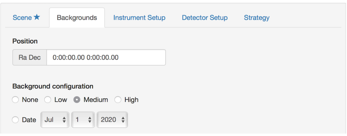
Background
NIRSpec observations are dominated by the detector noise, so the background is not a concern. Most of the time, you will be able to get a low background, but putting constraints on this parameter will lead to strong scheduling constraints, not benefiting to your observations. Keep it to medium to be conservative.
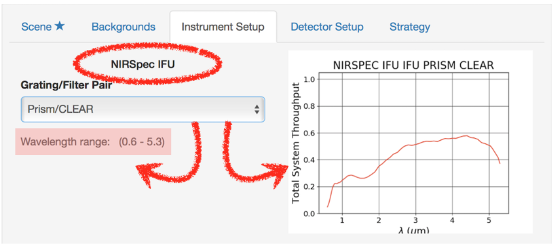
Instrument Setup
ETC reminds you what observing mode you are working with. You can select the combination of filter and grating needed: ETC will remind you of the wavelength range, and show you the corresponding throughput.
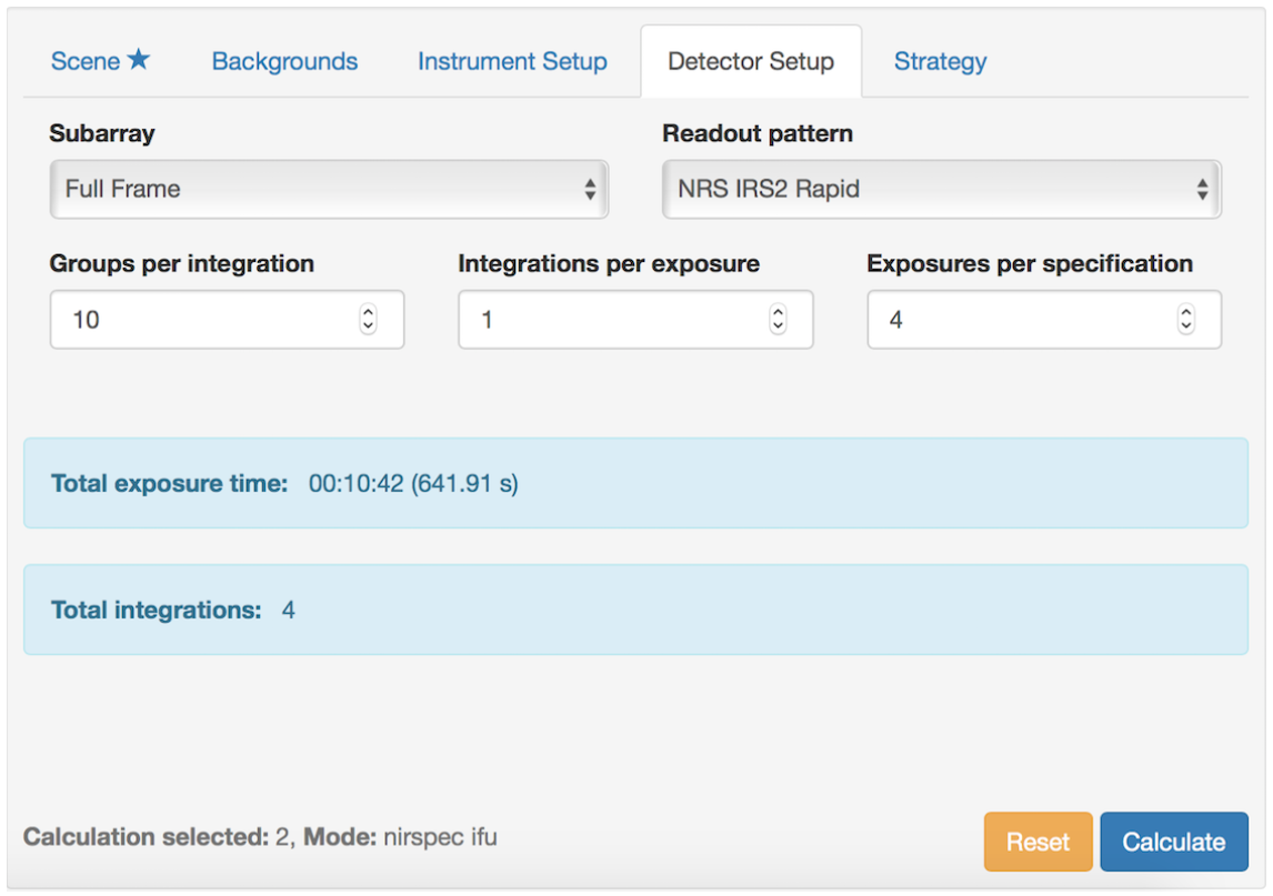
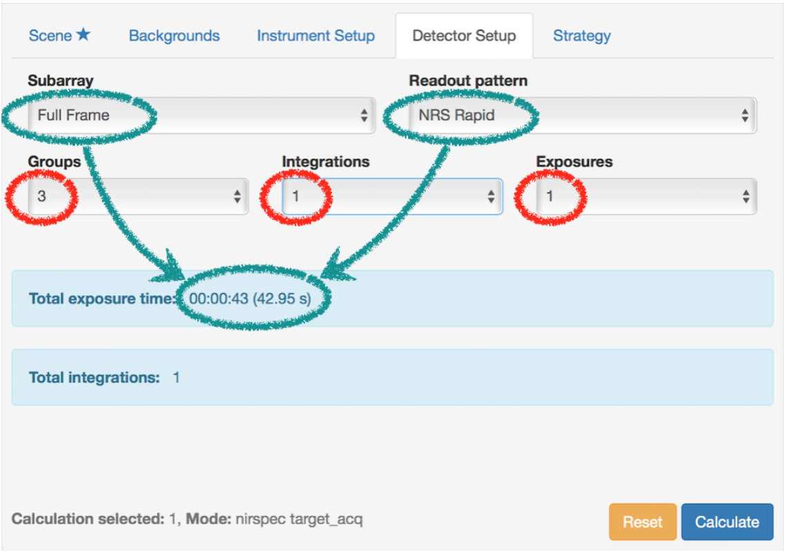
Detector Setup
You have to select parameters discussed in section NIRSpec in a nutshell.
Subarray: use Full Frame for small body observations.
Readout pattern: we have made the case that NRS IRS2 Rapid should be the best option, you can however select the one best suited for your observations.
Groups, Integrations, Exposures: as discussed previously, we select only one integration, and increase the number of groups until we reach the desired SNR, without reaching saturation. The number of exposures is set to 4 in order to mimic the 4-point nod strategy we want to set.
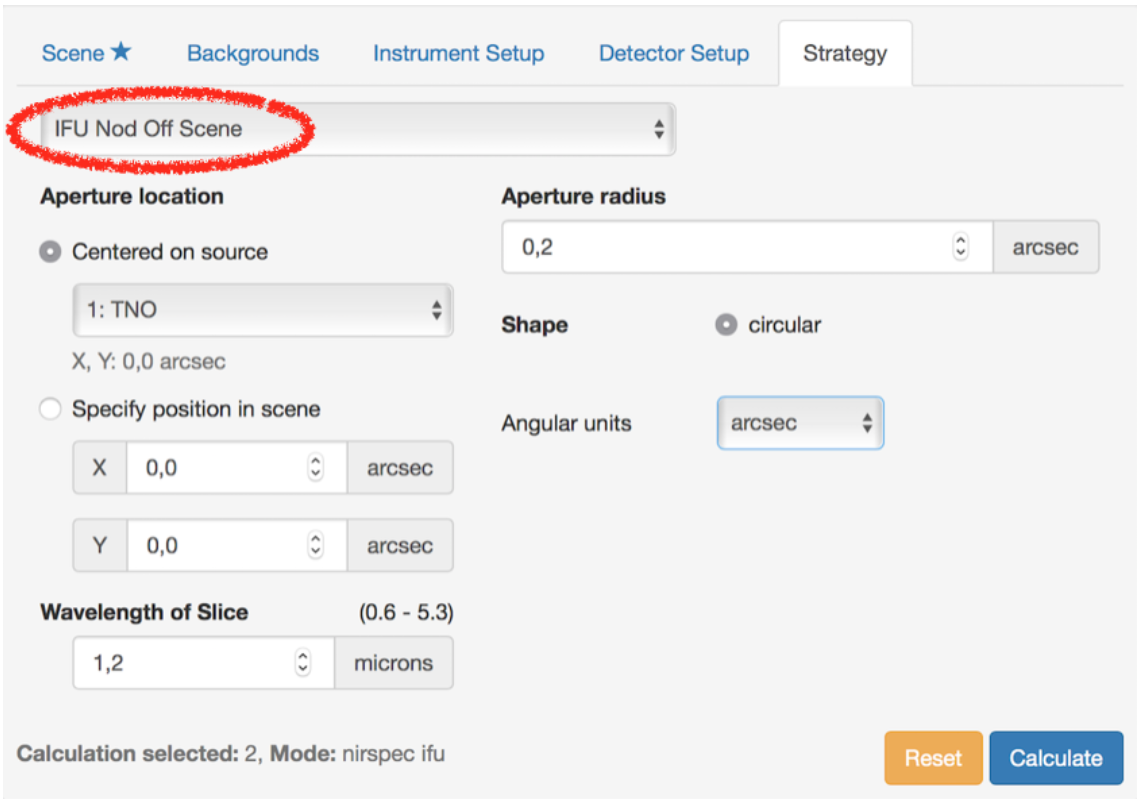
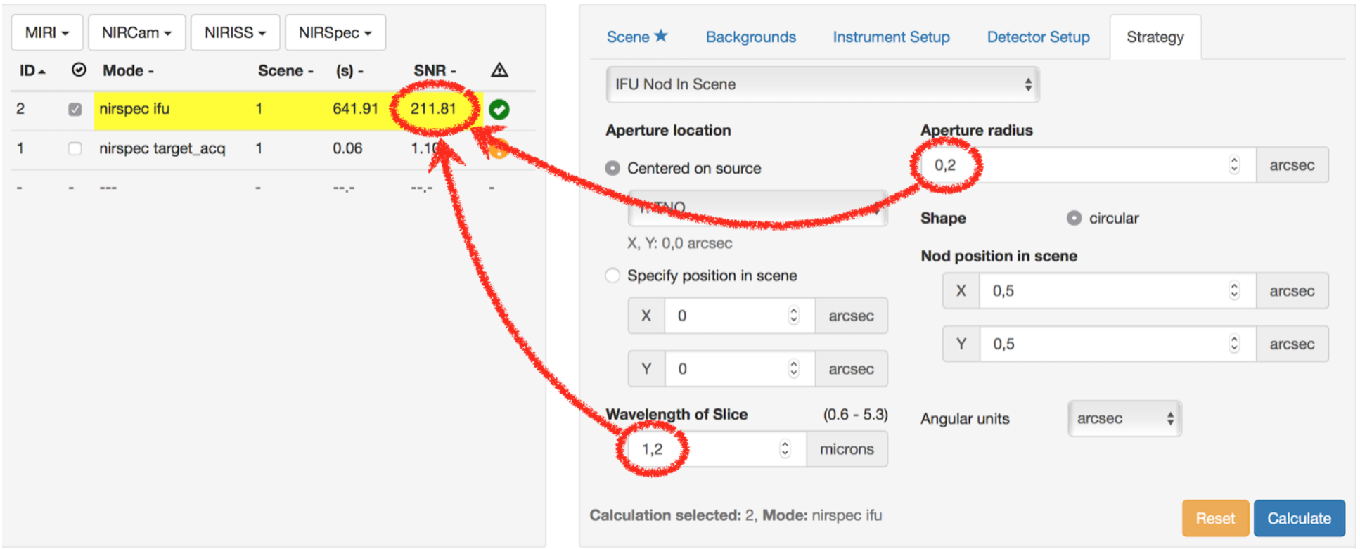
Strategy
Two nodding option are offered in the ETC: on-scene, and off-scene. Choosing one or the other will not have any drastic effect on the calculation (SNR is generally slightly lower with the off-scene nod, so this is the most conservative option). The on-scene option automatically sets the number of exposures to a multiple of 2. Thus, to set up a 4-point nod strategy, either select 4 exposures with an off-scene nod, or 2 exposures with an on-scene nod. You then set up the location and size of the aperture for extracting the signal, and define the wavelength of the slice for which the SNR will be computed.
Calculate
When you hit the Calculate button at the bottom, the ETC may take quite some time to actually perform the calculation. For instance, if your target is defined through a Phoenix Stellar Model rather than a Blackbody, calculations are going to take more time, since the model has a more complex shape with lines.
The summary of the calculation provided on the left-hand side shows a SNR: beside the readout pattern and the groups/integrations/exposures, this SNR is directly connected to the aperture radius and the wavelength of the slice you have chosen in your strategy. This is not the SNR of the whole spectrum, just the one for a given aperture at a given wavelength.
We find that an aperture of 0.2-0.3’’ is generally what provides a good SNR, otherwise too many pixels are involved in the calculation and the SNR drops. We also find that the wavelengths at which the best SNR are achieved are the following (keep in mind that the SNR computed at these wavelength are the maximum SNR achieved, they do not stand for the whole wavelength range):
- PRISM 1.20 µm
- 140H/M 1.15 µm
- 235H/M 2.00 µm
- 395H/M 3.20 µm
You can see this effect when you scroll down to have a look at the Images and Plots.
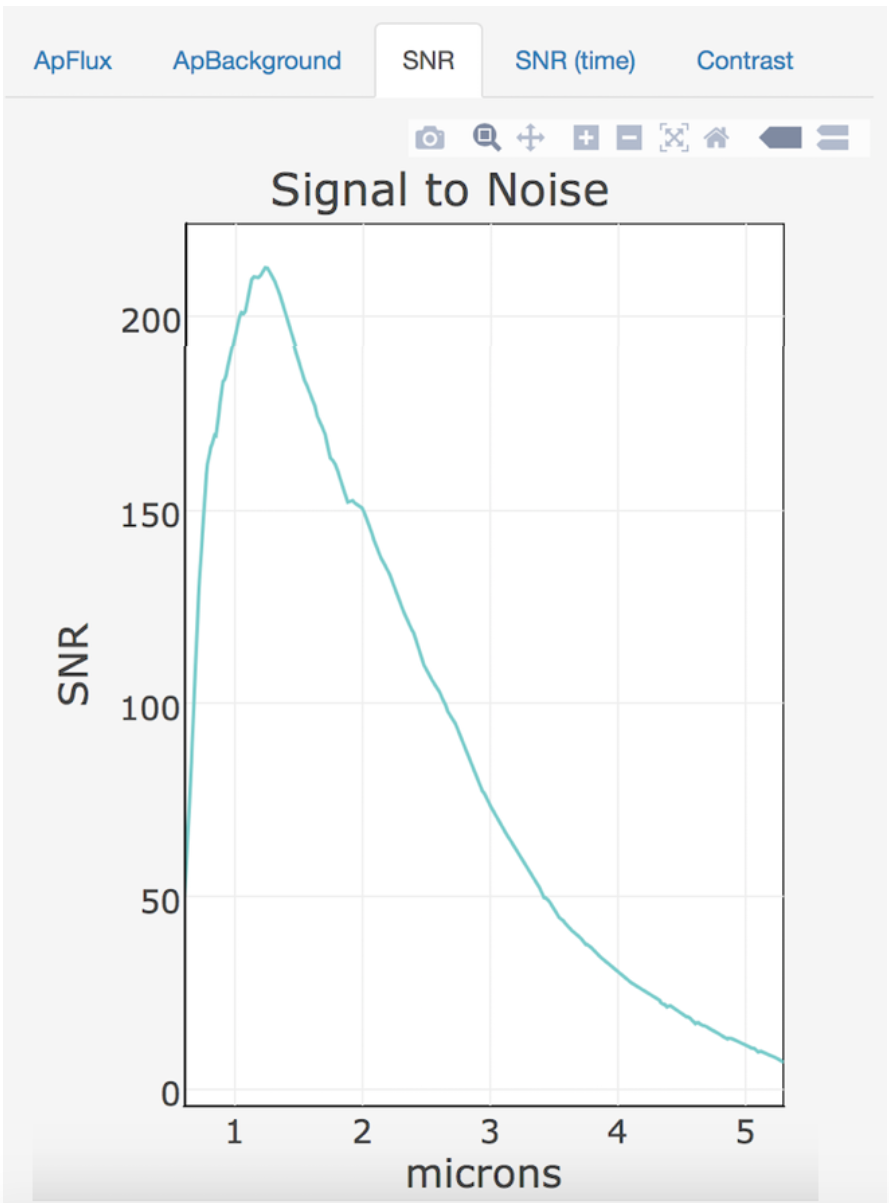
Plots will give you access to various information, like the flux in the aperture, the background, and the SNR, as a function of the wavelength. Small tools are available when you hover on the thumbnails.
You see in our example that although the maximum SNR is about 220 at 1.2 µm, it can drop significantly toward the longer wavelengths.
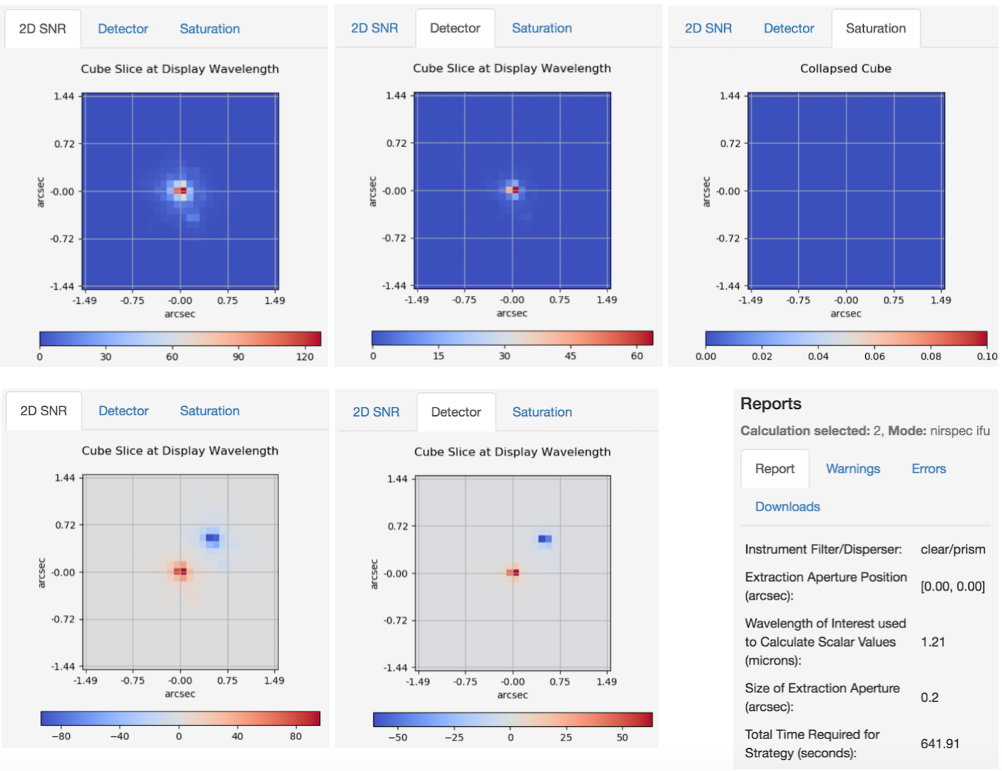
Images show you some other useful information, such as the 2D SNR of the scene, what the scene would look like on the detector, and the collapsed cube which helps locate the saturating pixels.
You can see in our example below that we do not saturate, but that the SNR may not be enough to separate the satellite from the main component of our target and actually get a spectrum from it.
Images from the on-scene nod will look quite different since exposures are subtracted from one another: you would get a positive and a negative image of the target, as shown below.
Finally on the right, reports are available to summarize your calculation, including warnings and errors if relevant. You can also download the products of the calculation, including the spectra, SNR curves etc.
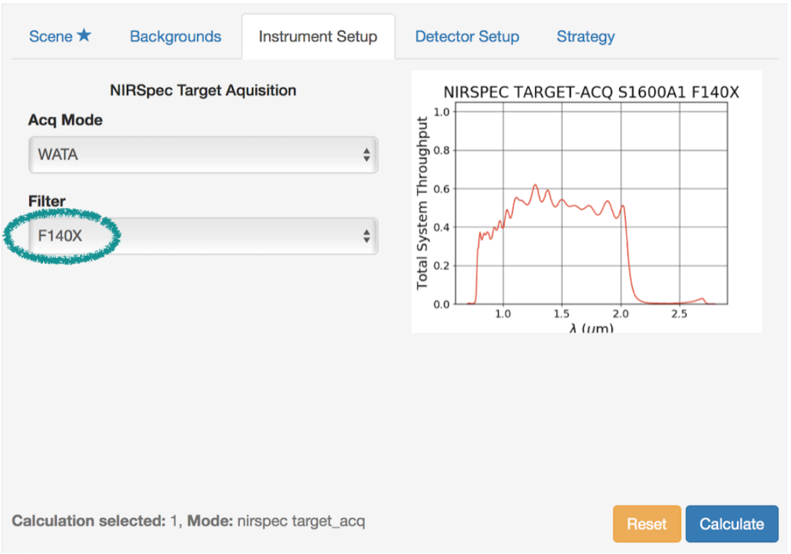
The case of Target Acquisition
The default and most effective mode for target acquisition is called WATA (Wide Aperture Target Acquisition). Calculations for TA are a bit particular in the sense that in the Detector Setup, the number of groups, integrations and exposures is already fixed and cannot be changed.
In order to reach the required SNR for the target acquisition to be successful (between 20 and saturation), you have to play with:
- the Filter (Instrument Setup),
- the Subarray (Detector Setup),
- the Readout pattern (Detector Setup).
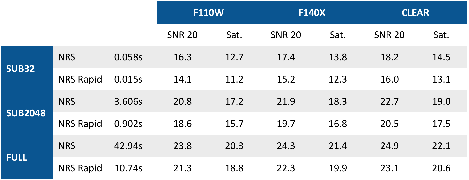
The table below provides a guideline (J magnitudes in Vegamag) for choosing the configurations best suited to your observation. In our example (V=19), two configurations can work:
- F110W + SUB2048 + NRS
- F140X + SUB2048 + NRS Rapid
Both do not yield the same exposure time though, but this parameter is not the dominant factor for the final time.
In general, using WATA takes between 10 and 15 minutes.
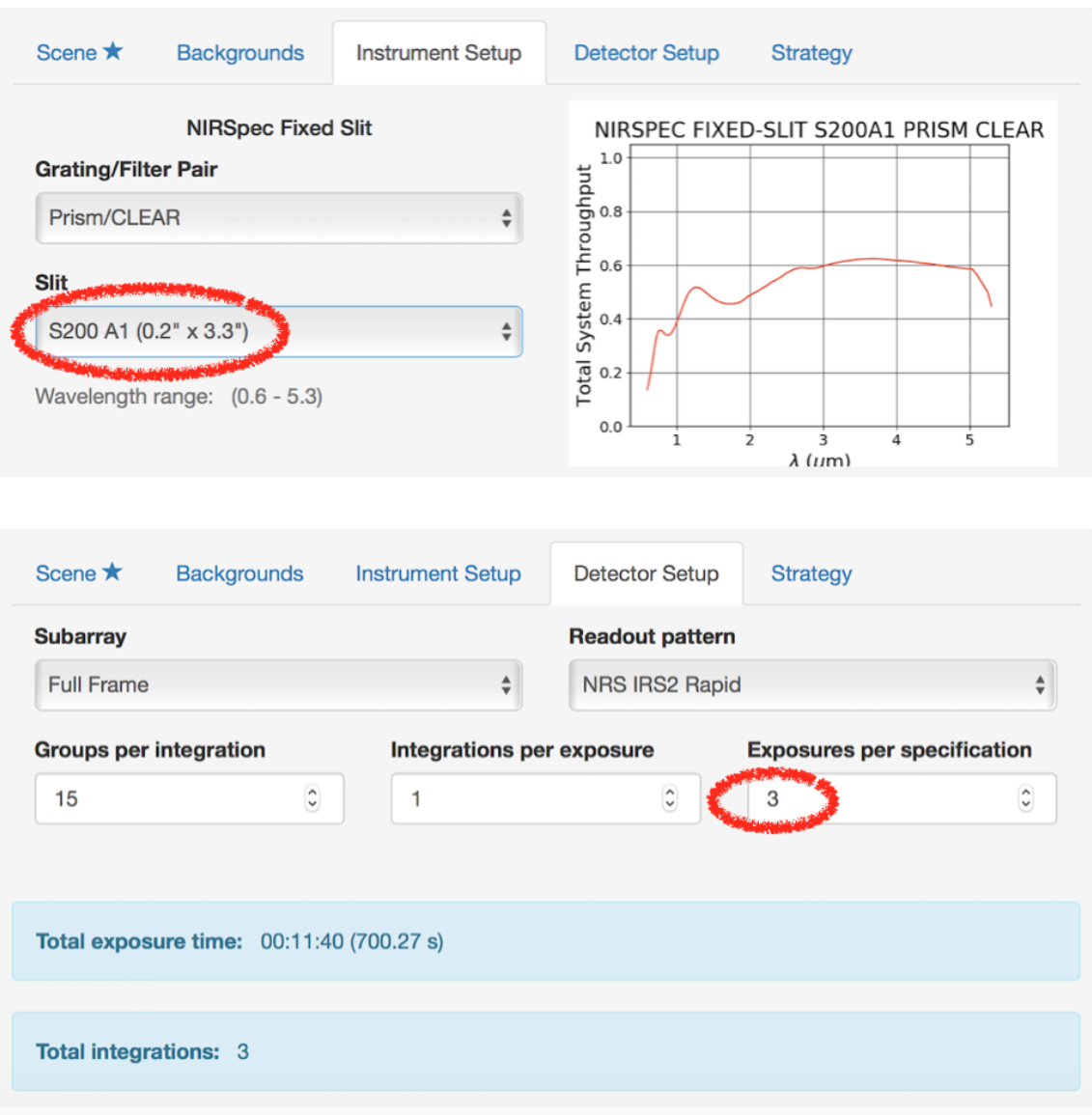
The case of Fixed Slit
When using the SLIT mode, defining your strategy is pretty much the same as for the IFU. In the Instrument Setup, you need to specify which slit you want to use.
In the Detector Setup, you should adapt the number of exposures to mimic the nodding strategy you want to use: either 2, 3 or 5 exposures. Similarly to the IFU mode, you should consider using one single integration, and increase the number of groups to increase the SNR, unless you reach saturation.
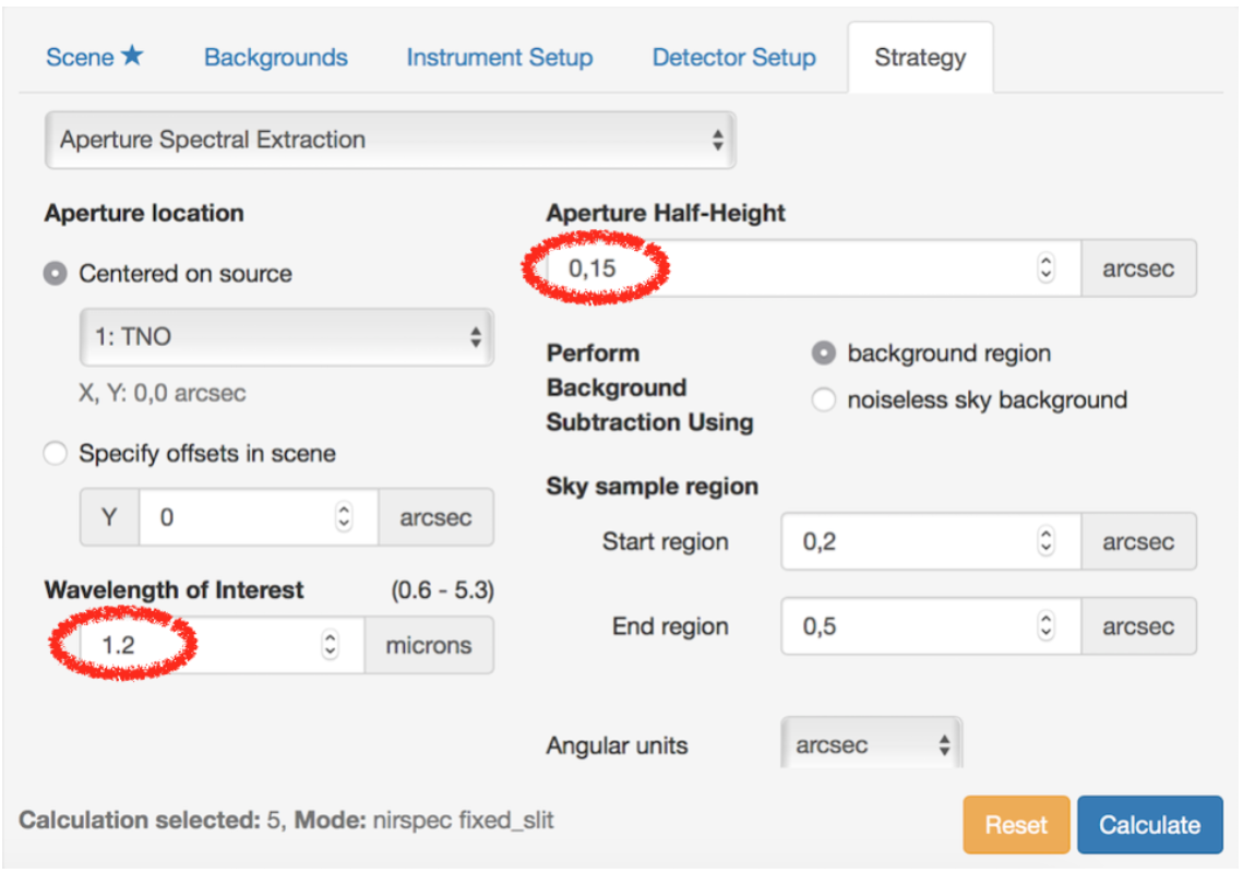
Finally, in the Strategy, you should adapt the wavelength of interest, as well as the aperture half-height which will be used in the SNR calculations. Note that the aperture half height should not be equal or larger than the slit size.
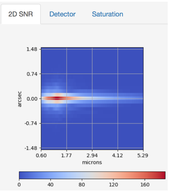
The Plots would look very similar as for the IFU, but the Images obviously are very different, as the IFU provides 3D cubes, while SLIT gives 2D images, as seen below.
A legitimate question arises: should you use the IFU or the SLIT? There is no straightforward answer, as several competing factors should be considered. NIRSpec is a detector-noise dominated instrument. This means that extracting a spectrum from an IFU cube involves more pixels, hence more noise. This is not a problem for bright sources, but for faint ones, it can easily decrease the sensitivity to the point where the loss of light in SLIT is overweight. However, using SLIT requires to use WATA, while this can be skipped for targets with a high-accuracy ephemeris in IFU. In addition, the IFU gives you the benefit of observing multiple systems without strong constraints on the instrument. Therefore, in order to choose the observing mode you need, you should try several options in both the ETC and APT, and make up your mind about the efficiency and the sensitivity you need.