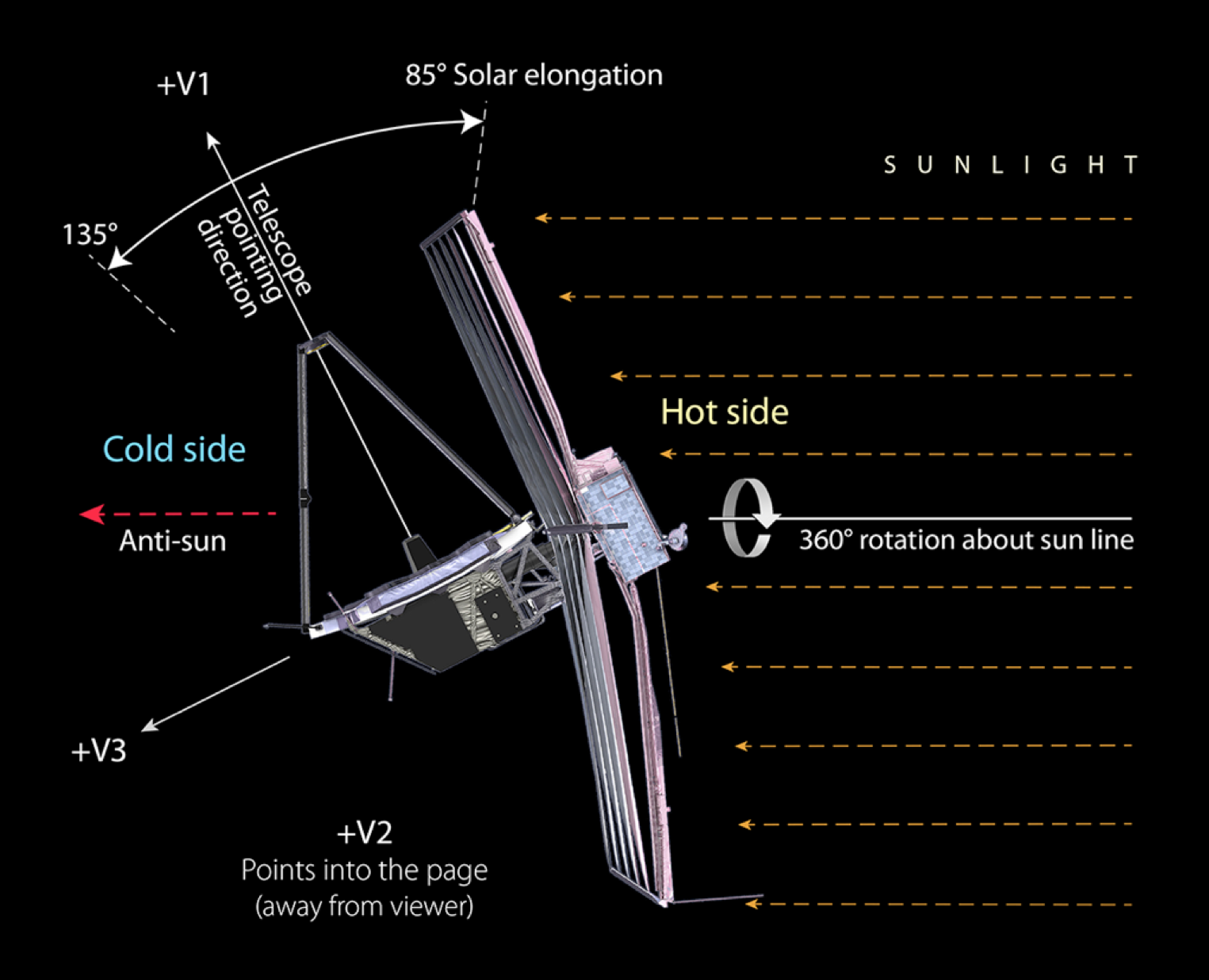
Because of its thermal design, JWST can only observe solar elongations between 85° and 135°. Please be sure to set up proper constraints in order to get the correct ephemeris for your target! Ephemeris for small bodies can be obtained on JPL/Horizons, by setting up @JWST in the observatory field. Please note that the current version makes use of a model of JWST’s orbit, which is not final yet and will be updated once the telescope is in space.

The telescope can track moving targets with a rate up to 30mas/s or 108’’/hr. Moving target observations will require slightly brighter guide stars (~1mag): one single guide star can last roughly 1hr.

Detectors — They are both HAWAII-2RG sensor chip arrays (SCAs) with 2048×2048 pixels of 18µm i.e. 100mas pixels on the sky, and a wavelength cut-off at 5.3µm. Four pixels on each side serve as electronic references to track variations of the input signal. There is a physical gap of 18’’ on the sky between the two SCAs: this implies a loss in wavelength in the IFU mode and the R=2700 gratings (because the spectra are long enough to span both detectors and are thus not recoverable). For other modes and gratings, the loss can be recovered with dithers and offsets on the target. Note: for bright extended objects like giant planets, subarrays are available: these are not useful for small bodies though, and are not discussed here.

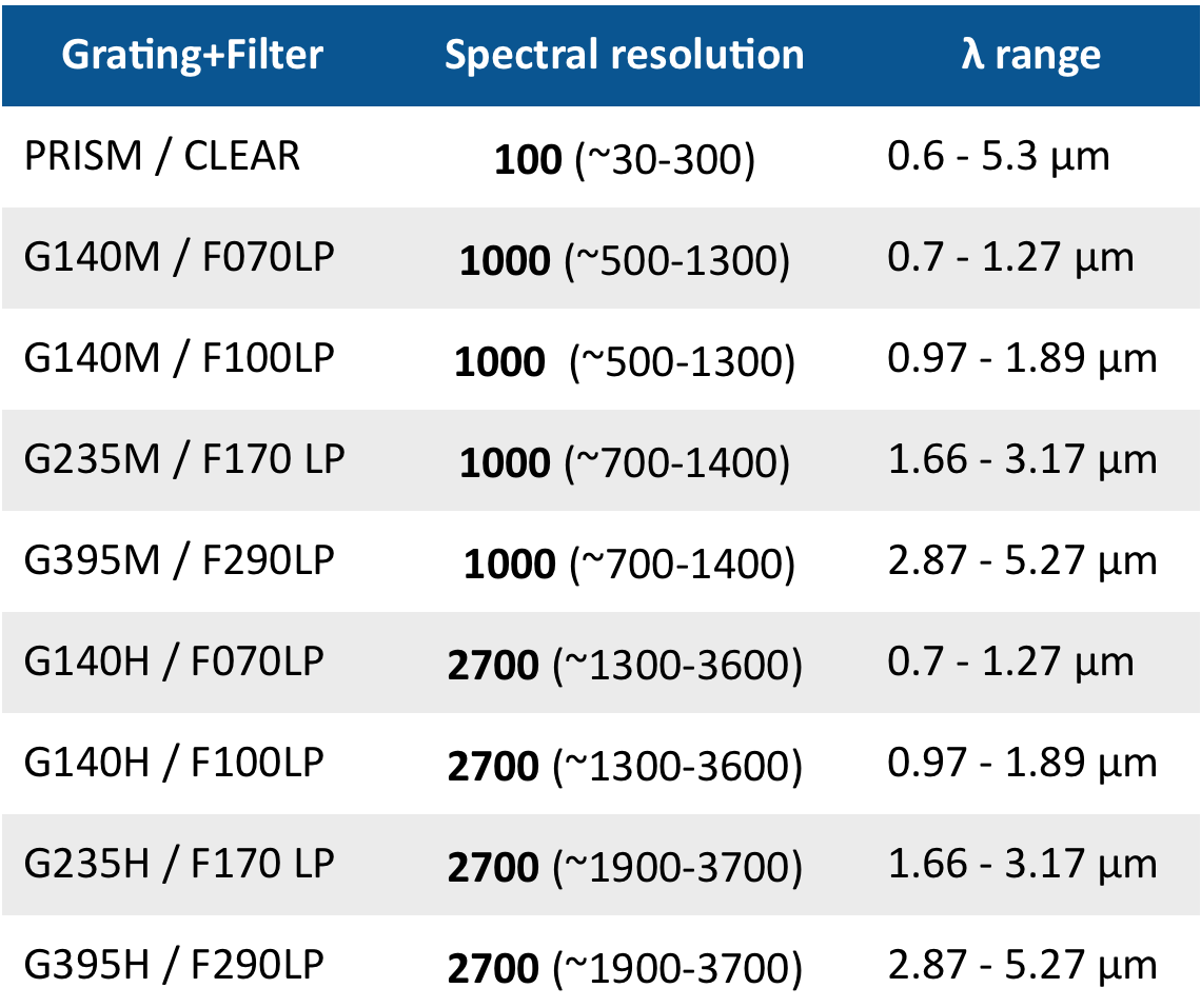
Wavelength coverage, spectral resolution and nodding — Filters and dispersers are available on two separate wheels, allowing for various combinations described below. In SLIT mode, 4 slits are available, plus one backup slit (S200B1):

• S200A1 − 0.2’’ × 3.2’’
• S200A2 − 0.2’’ × 3.2’’
• S400A1 − 0.4’’ × 3.65’’
• S1600A1 − 1.6’’ × 1.6’’

S1600A1 is optimized for observations of bright stars with transiting exoplanets in the NIRSpec time series mode BOTS.

Nods/dithers are available: 0, 2, 3 or 5 point nod along the slits.

In IFU mode, nods are separated by 2’’. All points of the 4pt nod lie within one IFU aperture of each other, so there is some overlap between fields.

The nod and dither patterns differ only for the processing, in particular for the background subtraction. Nodding is thus recommended as a preferred option.

Observing modes — NIRSpec can operate in several modes: MOS (multi-objects), IFU, SLIT and IMA (target acquisition only). IFU and MOS are mutually exclusive, while the slits can be used simultaneously with either MOS or IFU. The IFU is made of 30 slices for a total of 900 spaxels, the field of view is 3’’×3’’, with a 0.1’‘ sampling. The throughput is > 50% from 0.6 to 3.0µm, and > 80% beyond 3.0µm.

Choosing between SLIT and IFU is not straightforward. You usually loose some light from the target when using SLIT compared to IFU where the whole target is in the field. However, this can be overweight by the fact that SLIT can be more sensitive for faint sources, since it uses less pixels than IFU and thus introduces less detector noise. IFU can be used without target acquisition (WATA), while you will always need to use WATA for SLIT. Finally for multiple systems, IFU is much easier to schedule and operate.

Target acquisition (WATA) — In SLIT mode, it is required to use a target acquisition in order to place the object on the slits. However, this feature is not mandatory in IFU. Indeed, the aperture for target acquisition with NIRSpec is only 1.6’’, so the ephemeris of your target must be pretty accurate (you can check the uncertainty within the ephemeris files provided by Horizons). And in this regard, if the ephemeris is accurate enough that the target would fall in this small aperture, it should be accurate enough to fall in the 3’’×3’’ field of view of the IFU, thus reducing the need of target acquisition… The only remaining concern might be for the nods/dithers, which are separated by 2’’: if the target is not accurately centered, you might loose it while nodding.

If the uncertainty in the ephemeris is of the order of 1’’, we recommend that you do some astrometry on your target first, before scheduling NIRSpec observations.

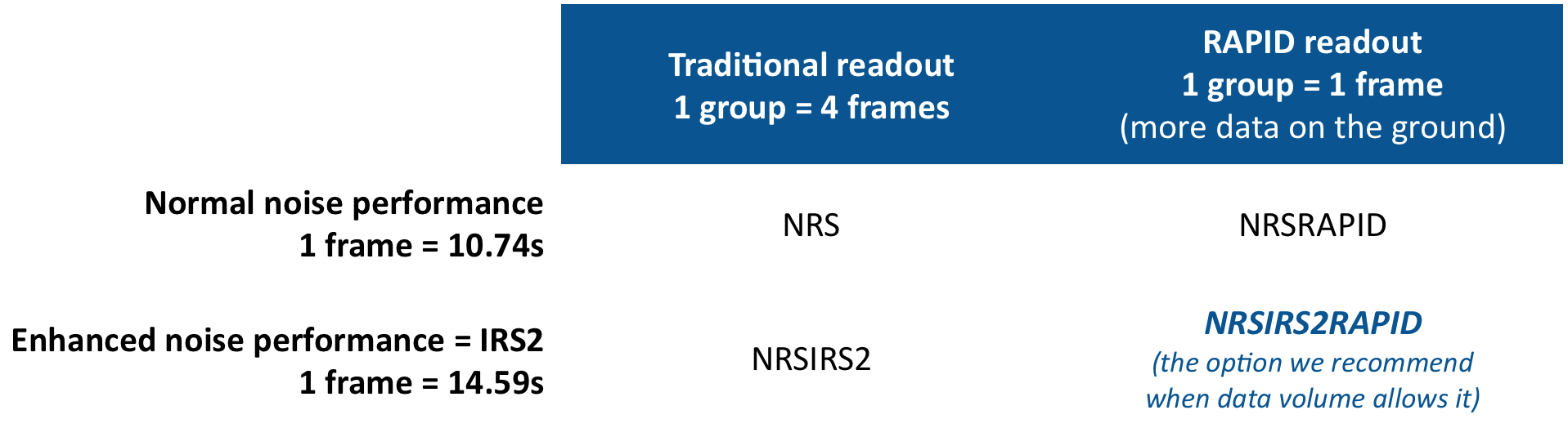
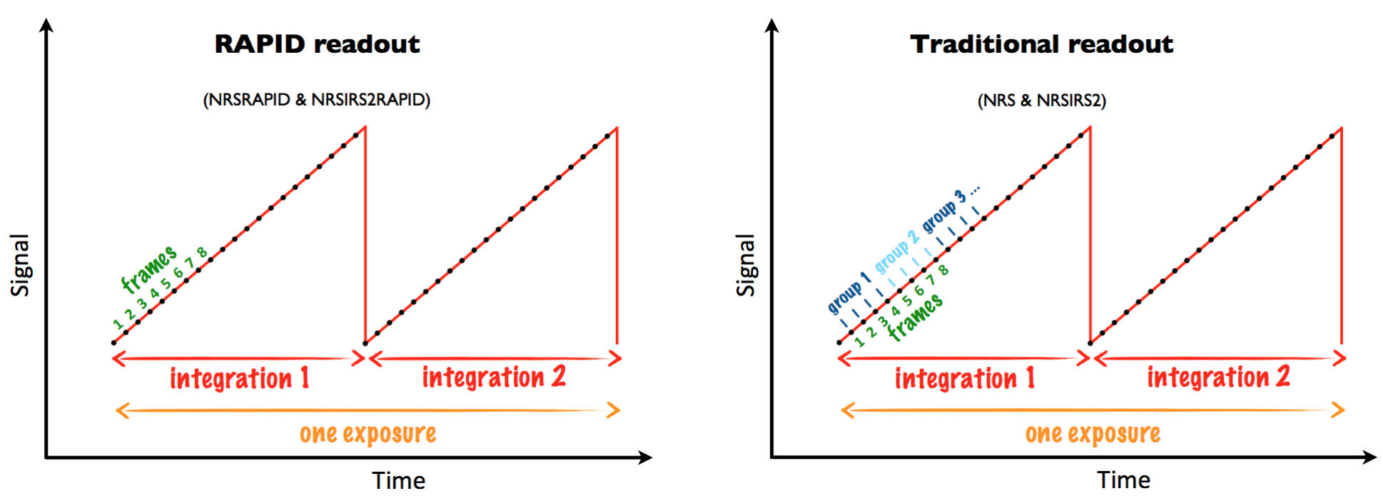
Readout modes — Each pixel can be addressed individually and read out in a non-destructive way. Two readout patterns are implemented: one traditional readout (NRS and NRS RAPID patterns) and one with an improved reference sampling and subtraction (IRS2, available in NRS IRS2 and NRS IRS2 RAPID patterns).

IRS2 interleaves sampling reference pixels with science pixels, thus improving the noise characteristics achievable during data processing. It helps for faint sources and in particular for long exposures on extremely faint objects. We therefore recommended to use the IRS2 readout modes, either through NRSIRS2 or NRSIRS2RAPID.

Readout and duration of a frame — As stated previously, each pixel can be addressed individually and read out in a non-destructive way multiple times during an integration: each non-destructive readout is called a frame. At the end of an integration, the pixel is read out a last time, then reset. In order to maintain the thermal stability of the instrument, pixels are read constantly at a fixed cadence which is set only by the readout pattern you have chosen (and also by the size of the subarray to be read, but this feature is not relevant here): either traditional (NRS and NRSIRS2) or RAPID (NRSRAPID and NRSIRS2RAPID). The duration of this frame is 10.74s for NRS and NRSRAPID, and 14.59s for NRSIRS2 and NRSIRS2RAPID.

Concept of frame/group/integration/exposure — We have seen that the pixels are read constantly at a fixed cadence. The output of each readout from this cadence is called a frame. For the normal patterns (NRS and NRSIRS2), a total of 4 frames are averaged to form a group. This group (=average of 4 frames) is the only output you will get to the ground, not the individual frames themselves. For the rapid patterns (NRSRAPID and NRSIRS2RAPID), 1 frame = 1 group. This is a way to get all the frames to the ground, but it also means that the data volume can increase severely

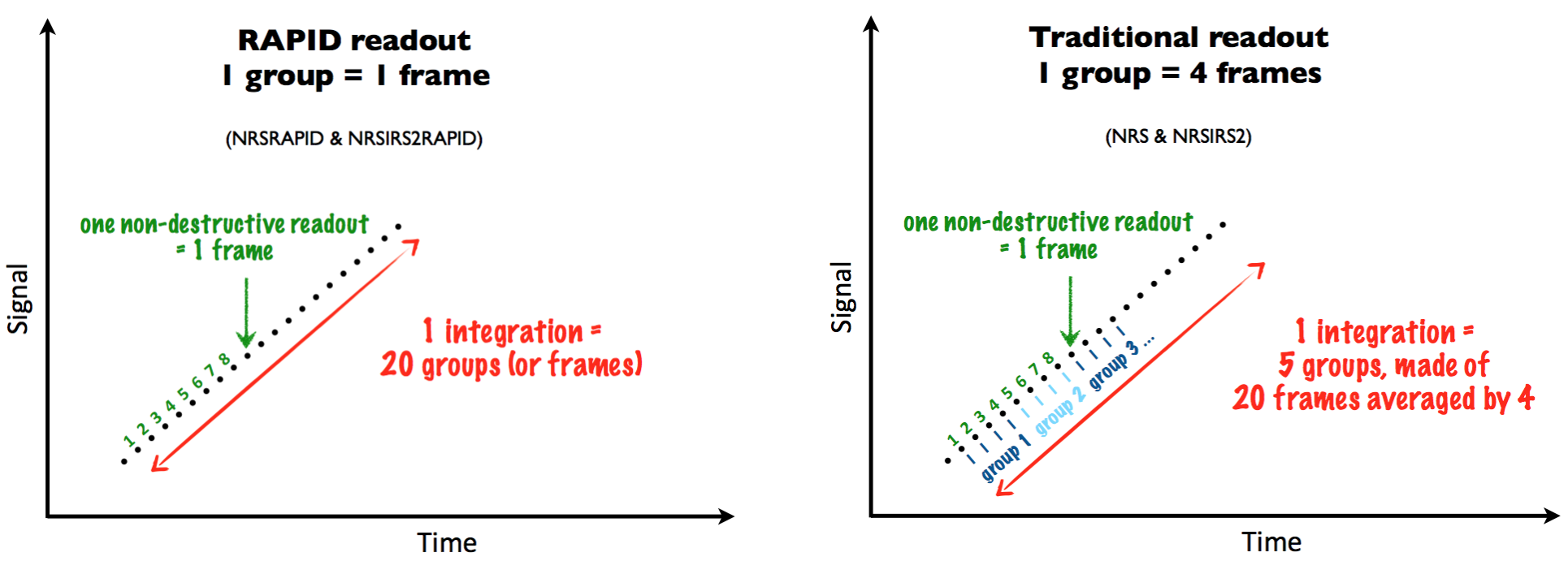
One integration is made of several groups, observed consecutively in an integration ramp: you get to tune the number of groups to be observed within one integration. Integrations are terminated by a reset.

We recommend to test the ETC with a trial and error procedure in order to reach the saturation limit: if the saturation is hit with x groups, then set your actual number of groups to x-1.

Multiple integrations can be observed without interruption in one single exposure. Once we have defined the number of groups per integration, if you still need to increase the total observing time, then increase the number of integrations per exposure. This is the best strategy for getting the highest signal to noise ratio. Indeed, several aspects need to be balanced:

• a single long integration can yield better noise performances, particularly on faint targets,
• the use of the RAPID patterns allows to remove frames affected by cosmic rays,
• using multiple integrations can also allow for improved cosmic ray correction,
• multiple integrations can limit hard saturation and provide time resolved spectroscopy.

If the required observing time is about 1000-1500s, and less than 3000s in general, we recommend to use exposures made of one single integration.

Note: in the ETC, there is no formal difference between integrations and exposures. In the APT though, there is a significant difference since both do not yield the same overheads. We will come back to this aspect in the following section.